Implement Your Own Control Loop
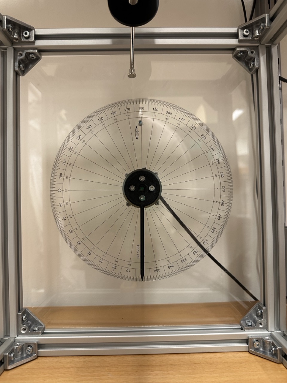
Here is a simple example showing how to use the Cloud Pendulum system in your own custom application. The CP system allows users to remotely run experiments on real robot hardware. The clients requests a "cell" to run their experiment on, and the server gives access to these cells whenever one is available. There are many types of experiments you can run on this system (e.g. simple pendulum, double pendulum, acrobot, pendubot etc.), each requiring a specific type of hardware in the cell. In this tutorial we will be using the DoubleIntegrator experiment type, which runs on cells that contain a single motor, like the one in the following picture. The GitHub code can be found here: https://github.com/cloudpendulum/getting_started.
Pre-requisite
The first step is to create an account on the cloud pendulum JupyterHub: https://cloudpendulum.m2.chalmers.se:1443/hub/signup. Once you sign up, contact one of the administrators to authorize your account. Once we authorize, you will be able to login into the system and write your own code for example, related to modeling, simulation, learning and control. During the authorization, you will also be provided with a user token with which you can do experiments on the real hardware.
Setup
To communicate with the server, we use the cloudpendulum client package. The documentation for this package can be found here: https://cloudpendulum.m2.chalmers.se/docs/.
from cloudpendulumclient.client import Client
The interface is built around the Client class, which handles the connection to the server. To start an experiment, the start_experiment method is used to ask the server to reserve a 'cell' for some period of time. We supply a user_token to this method which is used by the server to authenticate the user.
user_token = "YOUR USER TOKEN HERE"
You can find your user token in the 'user_token' by visiting File->Hub Control Panel->CP Token & Compute Status.
Let's try starting an experiment:
client = Client()
session_token, livestream_url = client.start_experiment(
    user_token = user_token,
    experiment_type = "DoubleIntegrator",
    experiment_time = 5.0,
    preparation_time = 5.0,
    record = True
)
print("Received response from server!")
print("Session token: ", session_token)
print("Livestream url: ", livestream_url)
print("Sleeping...")
import time
time.sleep(3.0)
print("Stopping experiment")
video_url = client.stop_experiment(session_token)
time.sleep(1.0)

# Show video
from misc import download_video
video_path = download_video(video_url)
from IPython.display import Video
Video(video_path)
When running the start_experiment, you may have received a response immediately, or it may have taken a while. The reason for this is that the server will wait to send the reply until it has successfully found an appropriate cell available to reserve for the client. If many clients are using the system simultaneously, some may have to wait for their turn.
From the start_experiment method, we get a session token and a livestream url. The session token is used by the server to authenticate all subsequent request relating to this experiment session, and the livestream url is used to view a live video feed of the experiment. The stop_experiment method is used to stop the experiment, as you would expect. If we had not used the stop_experiment method, the experiment would have stopped by itself after 5 seconds.
Since we specified record = True when starting the experiment, we get a video url from stop_experiment so that we can watch the experiment.
Controlling the motor
Now that we have reserved a cell from the server, let's do something a little bit more interesting; Let's control the motor! The motors are by default started in impedance control mode with proportional gain Kp and derivative gain Kd set to zero i.e. pure torque control. In this example we use set_position to set the position of the motor directly. We could also have used set_velocity or set_torque to set the velocity and torque of the motor respectively. We can use the get_position, get_velocity and get_torque methods to measure the position, velocity and torque from the motor.
import math
import numpy as np
import matplotlib.pyplot as plt

Tf = 5.0
client = Client()
session_token, livestream_url = client.start_experiment(
    user_token = user_token,
    experiment_type = "DoubleIntegrator",
    experiment_time = Tf,
    preparation_time = 5.0,
    record = True
)
print("Received response from server!")
print("Session token: ", session_token)
print("Livestream url: ", livestream_url)

# Set Kp, Kd for position control
kp = 0.04
kd = 0.001
client.set_impedance_controller_params([kp], [kd], session_token)

dt = 0.01
meas_dt = 0.0
meas_time = 0.0

print("Desired dt: ", dt)

n = int(Tf / dt)

meas_time_vec = np.zeros(n)
meas_pos = np.zeros(n)
meas_vel = np.zeros(n)
meas_tau = np.zeros(n)
meas_dt_vec = np.zeros(n)

i = 0

print("Running the control loop")
while meas_time < Tf and i < n:
    start_loop = time.time()
    meas_time += meas_dt

    ## Do your stuff here - START

    measured_position = client.get_position(session_token) # Measure position
    measured_velocity = client.get_velocity(session_token) # Measure velocity
    measured_torque = client.get_torque(session_token) # Measure torque

    # Send position command
    client.set_position(math.sin(meas_time), session_token)

    # Collect data for plotting
    meas_time_vec[i] = meas_time
    meas_pos[i] = measured_position
    meas_vel[i] = measured_velocity
    meas_tau[i] = measured_torque

    ## Do your stuff here - END
    i = i + 1
    exec_time = time.time() - start_loop

    while time.time() - start_loop < dt:
        pass
    meas_dt = time.time() - start_loop
    meas_dt_vec[i] = meas_dt

print("Finished")

video_url = client.stop_experiment(session_token)
time.sleep(1.0)

print("Average measured dt: ", np.mean(meas_dt_vec))

# Show plots
plt.figure
plt.plot(meas_time_vec, meas_pos)
plt.xlabel("Time (s)")
plt.ylabel("Position (rad)")
plt.title("Measured Position (rad) vs Time (s)")
plt.show()

# Measured Velocity
plt.figure
plt.plot(meas_time_vec, meas_vel)
plt.xlabel("Time (s)")
plt.ylabel("Velocity (rad/s)")
plt.title("Measured Velocity (rad/s) vs Time (s)")
plt.show()

# Measured Torque
plt.figure
plt.plot(meas_time_vec, meas_tau)
plt.xlabel("Time (s)")
plt.ylabel("Torque (Nm)")
plt.title("Measured Torque (Nm) vs Time (s)")
plt.show()

# Show video
from misc import download_video
video_path = download_video(video_url)
from IPython.display import Video
Video(video_path)
When running the start_experiment, you may have received a response immediately, or it may have taken a while. The reason for this is that the server will wait to send the reply until it has successfully found an appropriate cell available to reserve for the client. If many clients are using the system simultaneously, some may have to wait for their turn.
From the start_experiment method, we get a session token and a livestream url. The session token is used by the server to authenticate all subsequent request relating to this experiment session, and the livestream url is used to view a live video feed of the experiment. The stop_experiment method is used to stop the experiment, as you would expect. If we had not used the stop_experiment method, the experiment would have stopped by itself after 5 seconds.
Since we specified record = True when starting the experiment, we get a video url from stop_experiment so that we can watch the experiment.
Remarks
- The position tracking is not perfect. By selecting better Kp and Kd values this can be improved.
- It is difficult to achieve hard real time control in Python. So the control loop may terminate early and misses a few control ticks. This is usually not a problem but you may see the end point of the trajectory connected to zero. This is because we initialized our vectors with zeros.
Data Cleanup for Better Plotting
# Data cleanup for plotting because sometimes a few control ticks maybe missed
lastnonzero_index = np.max(np.nonzero(meas_time_vec)[-1]) + 1
N = int(Tf/dt)
print("Number of missed control ticks: ", N - lastnonzero_index)
meas_time_vec = meas_time_vec[:lastnonzero_index]
meas_pos = meas_pos[:lastnonzero_index]
meas_vel = meas_vel[:lastnonzero_index]
meas_tau = meas_tau[:lastnonzero_index]

# Show plots
plt.figure
plt.plot(meas_time_vec, meas_pos)
plt.xlabel("Time (s)")
plt.ylabel("Position (rad)")
plt.title("Measured Position (rad) vs Time (s)")
plt.show()

# Measured Velocity
plt.figure
plt.plot(meas_time_vec, meas_vel)
plt.xlabel("Time (s)")
plt.ylabel("Velocity (rad/s)")
plt.title("Measured Velocity (rad/s) vs Time (s)")
plt.show()

# Measured Torque
plt.figure
plt.plot(meas_time_vec, meas_tau)
plt.xlabel("Time (s)")
plt.ylabel("Torque (Nm)")
plt.title("Measured Torque (Nm) vs Time (s)")
plt.show()
Check your token status
You can check your token status using the get_user_info() method. Alternatively, you can visit File->Hub Control Panel->CP Token & Compute Status.
client.get_user_info(user_token) # Monitor the status of your user token